Random forest models explained
wnowak10
In previous posts, I explained decision trees, and how various algorithms search for optimal split points, given training features and label data. Popular decision tree libraries often go further, having the ability to construct forest classifiers. What are random forests and why are they so popular? Let’s figure this out:
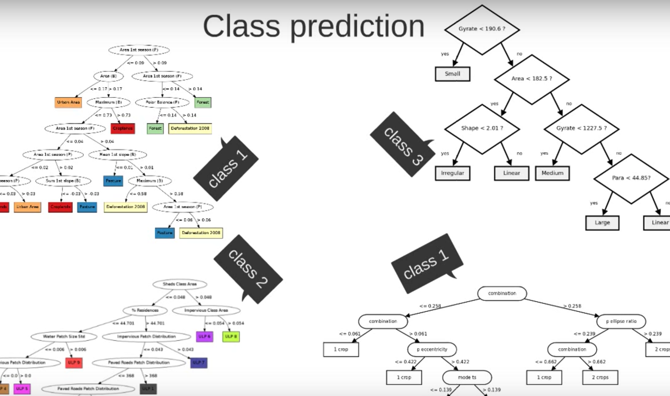
The idea of how random forests work isn’t so confusing. As I understand it, to construct a forest, we simply generate many trees. To build each tree, we select both a random subset of the training data, and a random subset of features that we choose to use as predictors (hence the moniker RANDOM). We construct many of these random trees to create a forest. In the end, we average (or in some other way) these individual, predictive trees to create a final model. This can be through a simple vote (that is, we look at the predicted class from each tree and accept the prediction with the highest vote total) or some other way. Thales Sehn Körting explains this well in his youtube video.
As I said, this isn’t so hard to understand. What is more elusive, I think, is why this process is as valuable as it is. We’ll need to dig deeper, and consider an example, to understand this. It should be pretty apparent, before we even begin, that random forests have an advantage with regards to scalability. Instead of searching through a full feature space and over all training data, forests simply construct many decision trees quickly (by using a subset of training data on a subset of all available features). In addition, forest construction can be done in parallel; for big data jobs, you could distribute tree construction to various machines and then, after, combine the results to generate your final forest model.
But the claim is that forests are superior for their classification accuracy, too. This is not immediately obvious. Our examples from before had only two features, which I fear won’t be too demonstrative here. So let’s create some more training data and see how a random forest would work, when compared to a vanilla decision tree.
Vanilla tree
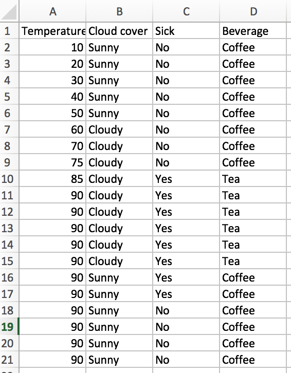
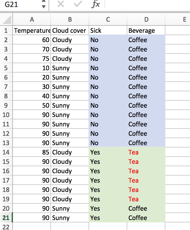
First, let’s look at the vanilla tree. How well does it do, and how computationally expensive is it? There are 20 training observations (n=20), and we have d=3 features. Since one of the features is numerical with 10 unique values, and the other two features are binary (cloudy or sunny, sick or not sick), our laborious information gain algorithm would have to check (10-1 + 1 + 1 = 11) potential split attributes. The best initial split is on “Sick”.
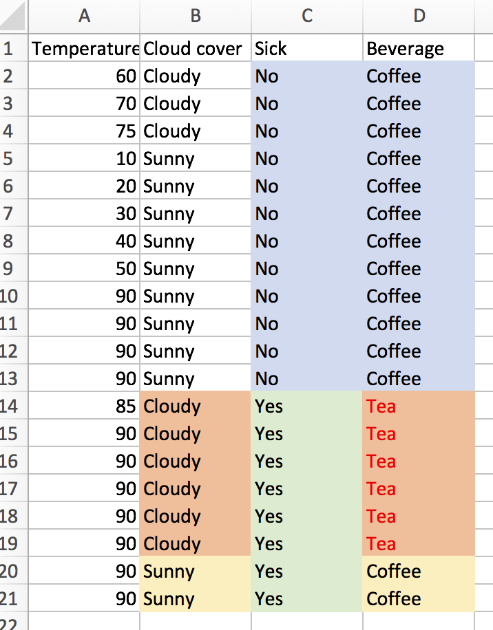
At this point, the we have one pure node. The entropy of the “Not Sick” node is 0, so we would code our algorithm to stop searching for a further split when we have reached this state. For the “Sick” node, we’ll still look for a second optimal split. We sort of lucked out, as there are only 2 unique temperature values (85 and 90), we only need to check 2 more potential splits (1 for the temperature feature and 1 for the cloud cover). We can easily see that splitting on “Cloudy” is the way to go.
After two splits, we have a pretty nice looking model. With a tree depth of 2, we have 3 pure end leaves. So how would the process work for a random forest? Could we achieve similar results?
Random forest
Let’s randomly pick 2 of our 3 features and we’ll randomly select 5 of our training observations. Let’s repeat this process 3 times and see what happens. My random generator produced {(1,2),(1,3),(1,3)}, so I’ll look at these features. After randomly selecting 5 rows, we find the following for our subsetted dataframes:
Subset 1.

For subset 1, the initial entropy is 0, so we don’t have to evaluate any split points. The same is true of subset 3!
For subset 2, we do have some “Tea” outcomes, so let’s consider the optimal split. There are 3 unique temperature values, and 2 outcomes for sick, so we need to check 3 (3- 1 + 1) potential split attributes. With a little consideration, we can see that splitting on sickness (or on temperature with the node between 60 and 90 degrees) results in the best information gain. If the individual is not sick, we have a pure leaf – coffee. If the person is sick, it is a toss up (50-50) if coffee or tea is the breakfast beverage of choice.
So, with this forest in place, let’s see how our model does at predicting. Without much work, we can see that it does pretty poorly. Since two of the trees purely predict coffee, and we only made a 3-tree forest, 2/3 of the votes will be for coffee, regardless of the feature inputs. This model will only be right 14/20 times.
So it seems that our forest was a bit small. We only looked at too few training obs or too few features. So I’ve still failed to convince anyone that forests do work with high accuracy. I suspect that my toy example was a bit too simplistic. Just like polling fails to work well when samples are too small, forests won’t work with too few training observations or features or trees. It would be a pain to manually work through another example with more trees and features, so let’s see if I can implement something in Python that makes the issue clear.
Elements of Statistical Learning by Hastie and Tibshirani, section 8.7, gives a nice discussion of what we are discussing here.
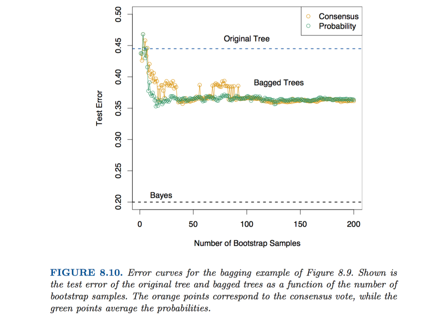
Let’s try to recreate and expand upon their example. They fabricate some data and then compare a tree to a forest. The key result that they find is shown in the following chart…
The error rate of the forest drops well below the test error rate for an individual tree, once the number of trees in the forest gets to ~10.
I was able to recreate the basic setup in R, but with some unexpected results. The full code can be found on github, here. But my basic tree model, constructing using R’s rpart package, tends to get around a 20-30% error rate, which is well below what they were finding in in ESL.
I first generated features using a helpful script from gung on stackoverflow (link here).
correlatedValue = function(x, r){
  r2 = r**2
  ve = 1-r2
  SD = sqrt(ve)
  e  = rnorm(length(x), mean=0, sd=SD)
  y  = r*x + e
  return(y)
}

# credit:
# http://stats.stackexchange.com/questions/38856/how-to-generate-correlated-random-numbers-given-means-variances-and-degree-of

n=30
x1 = rnorm(n)
x2 = correlatedValue(x=x1, r=.95)
x3  = correlatedValue(x=x1, r=.95)
x4 = correlatedValue(x=x1, r=.95)
x5 = correlatedValue(x=x1, r=.95)
Next, I need to generate the dependent variable. This was kinda a pain. I determined the list index for when variable x1 was above and below .5. Then, I replaced y (which was initially set to a vector of 0’s) values with sampled values, using the rule from the text:

outcomes=c(1,0)
BER = .2
greater=which(x1>.5)
less=which(x1<.5)
y=rep(0,n)
y[greater]=sample(outcomes,length(greater),replace = T,prob = c(1-BER,BER))
y[less]=sample(outcomes,length(less),replace = T,prob = c(BER,1-BER))
y
I next built the tree, using rpart:
# Classification Tree with rpart
library(rpart)
library(rpart.plot)
# grow tree
fit <- rpart(y ~ x1 + x2 + x3 +x4+x5,
             method="class", data=train_df
             , minbucket=5)

fit
rpart.plot(fit,type=0)
Finally, I also generate test data.
test_x1 = rnorm(2000)
test_x2 = correlatedValue(x=test_x1, r=.95)
test_x3  = correlatedValue(x=test_x1, r=.95)
test_x4 = correlatedValue(x=test_x1, r=.95)
test_x5 = correlatedValue(x=test_x1, r=.95)
test_features=data.frame(test_x1,test_x2,
                         test_x3, test_x4,
                         test_x5)
colnames(test_features)=c('x1','x2','x3','x4','x5')
head(test_features)
test_greater=which(test_features$x1>.5)
test_less=which(test_features$x1<.5)
test_y=rep(0,n)
test_y[test_greater]=sample(outcomes,length(test_greater),replace = T,prob = c(1-BER,BER))
test_y[test_less]=sample(outcomes,length(test_less),replace = T,prob = c(BER,1-BER))
test_y
sum(test_y)
I should explain the BER variable. In ESL, they note that the Bayes Error Rate of this model is .2. If you check out the construction of y and test_y, you should see that this makes sense. Basically, there is some signal in our dependent variable, but 20% noise, too. That is, if the x1 variable is above .5, y = 1 with probability .8 (= 1 - BER). If x1 < .5, y = 1 with probability .2. So the construction model is pretty simple. We should have one split for x1. If x1 < .5, predicting 0 is our models’ best bet, and if x1 > .5, we should predict 1.
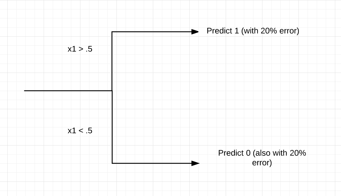
This correct and parsimonious model will never reliably do better than an error rate of 20%, as we built this pure randomness into the model.
Then, to use R’s predict function, I had to make sure that the variable names in the test set were the same as in the training (x1, x2…). I rename with the colnames() function.
p=predict(fit,newdata=test_features,type="vector")
# codes 0s as 2s for some reason
# run this in order!
p=replace(p, p==1, 0)
p=replace(p, p==2, 1)
head(p)
head(test_y)
sum(p==test_y)/length(p) # test error!
Running all this code often shows that my single tree results in an error of ~30%, which is less than the authors find (seen above in Tree vs forests error chart). I repeated this process 100 times, and a histogram shows a wide spread, but an average error rate for a single tree of ~20-40%.
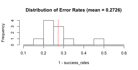
So, I need to figure out why my test error tends to be smaller than HT&F found. An open question, at the moment. Please leave comments in comments section!
Nevertheless, let’s continue on with our original purpose. I wanted to see the empirical results of forests, versus trees. Let’s run some experiments and see how we fare when we begin to tweak the model and/or parameters.
Trees versus forests
I ran similar code, using R’s randomForest function. Alas, the results are not good. With 1 tree in the forest, I find an average error rate that is far different from my rpart tree constructed above. Shouldn’t a 1 tree forest = a tree? I am unclear why the different exists. We also see that the variance of forest models with 1 tree is well below the variance of my rpart tree models above. Forest should have lower variance, but again, not this 1 tree forest. Something is askew.

Another problem is that there is essentially no difference in the model as the number of trees in the forest increases. Below is a histogram showing the test error rates on 100 simulations. This looks nearly identical to the histogram showing the error rates for a 1 tree forest. WTF?
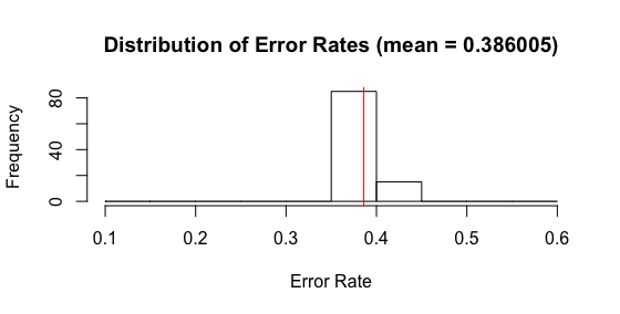
Clearly, there’s some misunderstanding on my part. Bummer. I’ll try to work through it and update you all as I go. This post has grown a bit long and needs to be pruned :), so I think it’ll probably be best to conduct some further debugging in further posts. I’ll link to those here, as they are created.
(FYI, here is the R code for the forest model creation and histograms:)
# randomForest
# a function to return correlated variables
correlatedValue = function(x, r){
  r2 = r**2
  ve = 1-r2
  SD = sqrt(ve)
  e  = rnorm(length(x), mean=0, sd=SD)
  y  = r*x + e
  return(y)
}

# create training data
make_train_data = function( n){
  #n=30 # number of variables in training set
  x1 = rnorm(n) # random normal, mean 1, sd 1
  x2 = correlatedValue(x=x1, r=.95) #4 other correlated features
  x3  = correlatedValue(x=x1, r=.95)
  x4 = correlatedValue(x=x1, r=.95)
  x5 = correlatedValue(x=x1, r=.95)

  # create label variable.
  outcomes=c(1,0)
  BER = .2 # bayes error rate of 20%
  greater=which(x1>.5)
  less=which(x1<.5)
  y=rep(0,n)
  y[greater]=sample(outcomes,length(greater),replace = T,prob = c(1-BER,BER))
  y[less]=sample(outcomes,length(less),replace = T,prob = c(BER,1-BER))

  # bayes error = .2 because y
  # is symmetric with a bayes error of .2. if we had a<.5 and
  # p(y=1|x>.5)= .5 and P(y=1|x<.5) = .7, then bayes error would be
  # average of .5 and .3 = .4. ya? ya.
  train_features=data.frame(x1,x2,x3,x4,x5)
  train_df=data.frame(x1,x2,x3,x4,x5,y)
  train_df$y=as.factor(train_df$y)
  return(train_df)
}

# generate random test features
make_test_features = function(n){
  #test_n=2000
  test_x1 = rnorm(n)
  test_x2 = correlatedValue(x=test_x1, r=.95)
  test_x3  = correlatedValue(x=test_x1, r=.95)
  test_x4 = correlatedValue(x=test_x1, r=.95)
  test_x5 = correlatedValue(x=test_x1, r=.95)
  test_features=data.frame(test_x1,test_x2,
                           test_x3, test_x4,
                           test_x5)
  # rename cols so they match 'fit' model
  colnames(test_features)=c('x1','x2','x3','x4','x5')
  return(test_features)
}

# generate test y values, given features
make_test_label=function(features,n){
  outcomes=c(1,0)
  BER=.2
  test_greater=which(features$x1>.5)
  test_less=which(features$x1<.5)
  test_y=rep(0,n)
  test_y[test_greater]=sample(outcomes,length(test_greater),replace = T,prob = c(1-BER,BER))
  test_y[test_less]=sample(outcomes,length(test_less),replace = T,prob = c(BER,1-BER))
  return(test_y)
}

# return success classified rate for forest model
forest_prediction= function(numTrees)
{
  # Classification Tree with rpart
  library(randomForest)
  train_df=make_train_data(30)
  forestFit <- randomForest(y ~ x1 + x2 + x3 +x4+x5,
                            data=train_df,
                            ntree=numTrees)

  tfs=make_test_features(2000)
  test_labs=make_test_label(tfs,2000)

  # how does model do on test data? what is error?
  p=predict(forestFit,newdata=tfs,type="response")
  # codes 0s as 2s for some reason
  # run this in order!
  p=replace(p, p==1, 0)
  p=replace(p, p==2, 1)
  head(p)
  head(test_labs)
  return(sum(p==test_labs)/length(p)) # test success!
}


success_rates=c()
for(i in seq(100)) {
  success_rates=c(success_rates,forest_prediction(5))
}
success_rates

title=sprintf("Distribution of Error Rates (mean = %s)", mean(1-success_rates))
hist(1-success_rates,breaks=seq(.1,.6,.05),
     main=title,xlab="Error Rate")
abline(v=mean(1-success_rates),col="red")
