A beginner's guide to decision tree algorithms
wnowak10
This is the first part of a series where I intend to explain how decision trees work. In this, I will cover part 1. Parts 2-5 will be in subsequent posts.
- Part 1: A beginner’s take on decision trees and splitting strategies.
- Part 2: How do vanilla tree algorithms even work?
- Part 3: Why random forests are useful and what ensembles are
- Part 4: How gradient boosting applies
- Part 5: What bagging is
If you need a primer on what a decision tree is, there is a lot of good extant content on this. Check out this simple video for an explanation of the basic idea.
Also, be aware that, in this section, I’ll try to first explain it in my own words, using my own generated ideas. This might mean that I use notation that differs from best practice. But, I find that it can often help me to think through problems on my own first, before delving into the literature and reading about best practices. Of course, though, I will do this too. You can find that in Part 2.
Table of contents:
-
Section 1.1 Categorical dependent variables
-
Section 1.1.1 Numeric features
-
Section 1.1.2 Categorical features
-
Section 1.2 Numerical dependent variables
I will first talk about categorical dependent variables in section 1.1. I’ll talk about using decision trees for numerical dependent variables in section 1.2.
1.1 Categorical dependent variables
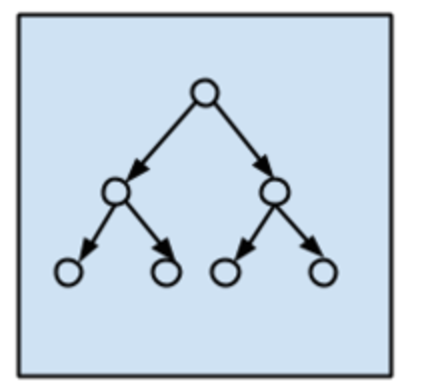
We’ll assume that this dependent variable is a binary random variable. And we’ll also assume that our trees will only have two branches emanating from each node. E.g.
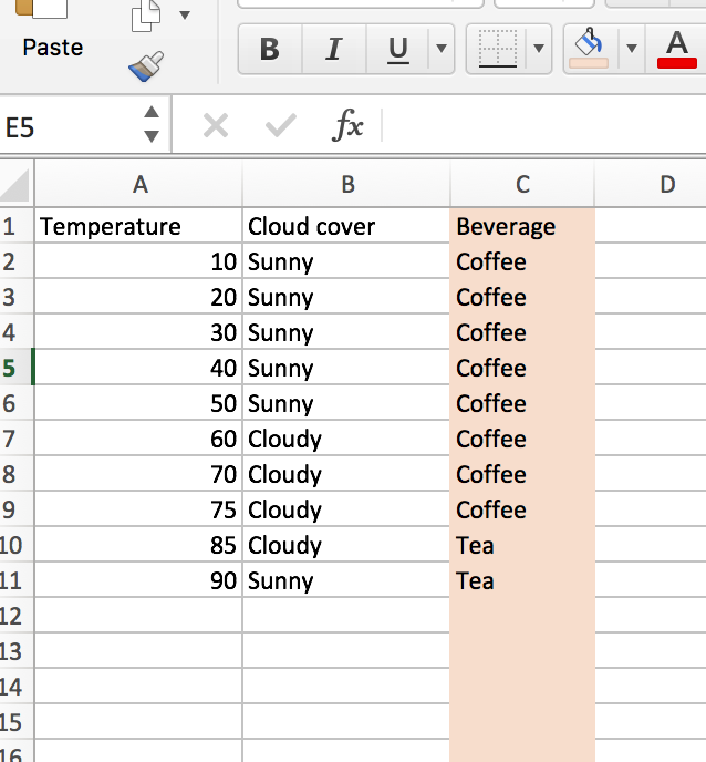
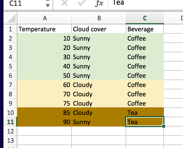
My understanding is that vanilla decision trees work by looking at data (which can be categorical or quantitive in nature), and finding the most information-rich split (more on this later). For example, if I were trying to classify “Beverage” using “Temperature” and “Cloud cover” as classifiers (as shown in the following table),
what would be the optimal first split for the tree?
Actually, did you think about it? Hopefully.
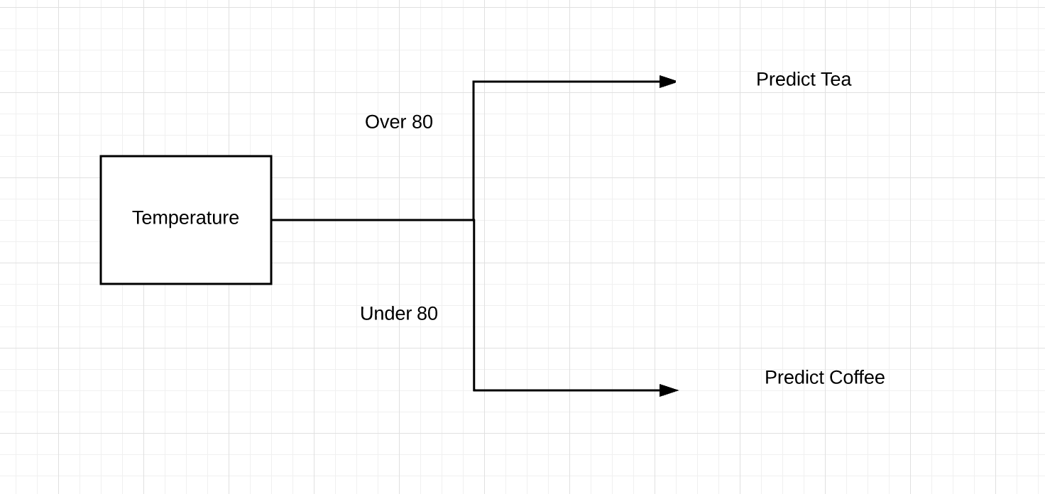
We can see that splitting on the temp is the best call, as if temps are below 80, we can correctly bin every beverage choice. We don’t even need the information provided about the cloud cover.
This basic split shows the “tree” idea:
To sum up, Wikipedia gives some semi-helpful pseudo-code that explains the decision tree process (though the gory and exciting details are absent).
- Check for the above base cases.
- For each attribute a, find the normalized information gain ratio from splitting on a.
- Let a_best be the attribute with the highest normalized information gain.
- Create a decision node that splits on a_best.
- Recur on the sublists obtained by splitting on a_best, and add those nodes as children of node.
It still remains to be seen: how does the computer actually do this? In particular, how do they determine that attribute “a” has the highest information gain?
Assume that there are p features. There n observations in our training set that we must classify. We need to determine:
- Which of the p features is best to split on? Where do we split this feature (if it is numeric or categorical with more than 2 outcomes)? (I’ll refer to this as the attribute (a) that we split on. That is, referring to an attribute a describes both the feature and the split point of that feature.)
We are trying to classify a label, which can take values 1 or 0. (In the example above, we had p = 2 features, and we could easily see that splitting on the temperature feature at some point between 75 and 85 was the right move. So we need to look at each feature and then describe, numerically, how well this split does in terms of helping us acheive our end goal of classification.
For numeric features:
Classification of split:
It seems that it’d be wise to sort the data on the numeric variable. Using our example, this would be temperature. Looking at the table above, we’d split somewhere like 55 (the median of the temperature set). If we did this, we’d find that 100% of beverages below 55 are coffee, and 60% (3/5) of beverages above 55 degrees are coffee.
Ideally, in a pure split, we’d have both nodes of the split at 100% (this would mean there is no ambiguity in the classification).
One idea for a helpful numerical descriptor could be s, where s = b1 + b2, where b1 = max(x, 1-x) with x = sum(li)/(c1), where li is the ith label and c1 is the number of elements in branch 1 (c for cardinality). b2 is defined similarly for the second branch.
In this case, splitting on feature “Temperature” at the median, we find that saQ2 = 1 + .6 = 1.6. It seems that an ideal split would result in two pure splits, leaving us with s = 1 + 1 = 2. On the contrary, a non-informative split would do no better than chance. In binary classification, this should result in 50% success along each branch. So, we have 1 < s < 2.
Pseudo-code for the optimal classification for a numeric feature would look something like:
- Set m = 0.
- Sort data by numeric feature
- Set attribute = median (Q2).
- Calculate s for this split. If s > m: m = s. If s < m, stop.
- If s does not equal 2, test a new attribute according to rule r.
- Repeat 3 and 4.
RULE R
*If b1 > b2, move test new attribute = median of upper half of data. If b1 < b2, move to new attribute = median of lower half of data.
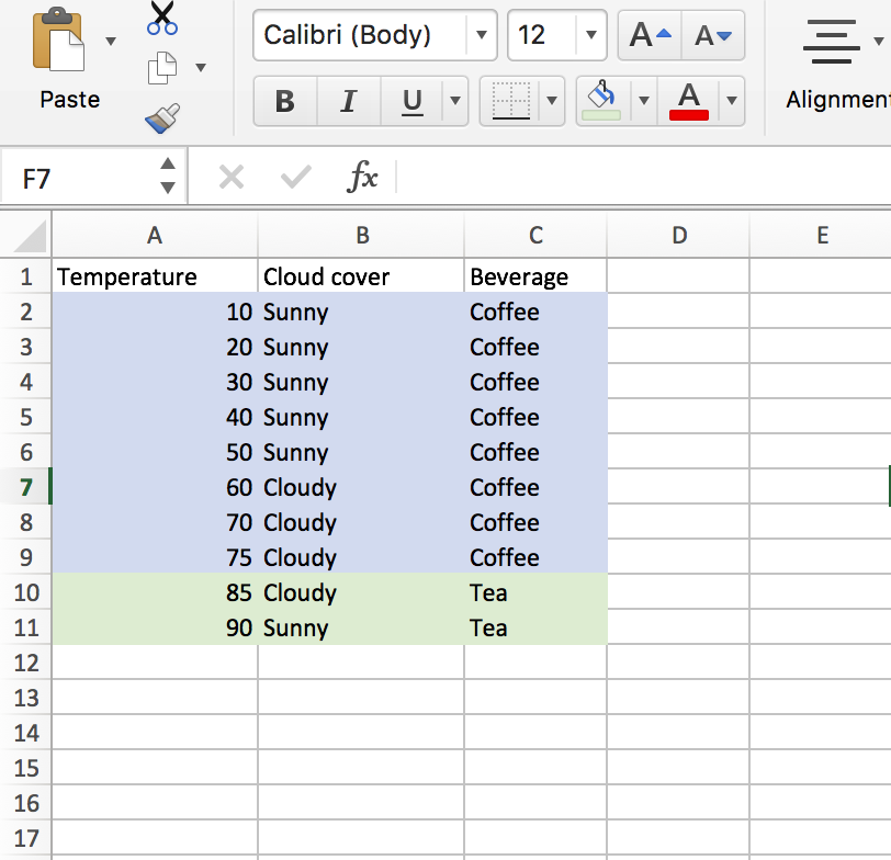
Let’s continue with the coffee and tea example. Following rule r, we’d choose a new attribute which is the median of upper half (since b1>b2). In this case, the median is 75. If we bin everything up to and including 75, we get the following.
Now, we find that s = 1 + 1 = 2. Since we have reached the maximum 2, we can stop our search.
Split choice:
In addition to judging our split attribute on its ability to successfully classify, we can generate another metric to judge various split attributes.
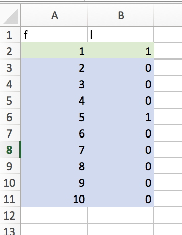
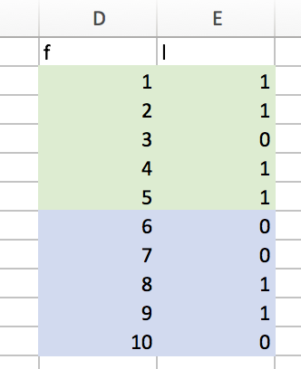
A good attribute splits data evenly. In example 1 below, the attribute acheives an s score of 1 + .89 = 1.89. However, it doesn’t split the data very evenly.
- Example 1:
In example 2, we have a worse split, in that s = .8 + .6 = 1.4.
- Example 2:
However, we are “doing more work” here. Given that we are trying to productively classify all data points, an attribute that produces a more even split should be prized for its efficiency, in some sense. We will have to rely on fewer nodes of a decision tree if each node can more evenly split the data.
We can now introduce another metric. We will call this metric e. e = log(c1) + log(c2). For example 1, we find e1 = log(1)+log(9) = .954. In example 2, e2 = log(5)+log(5) = 1.379.
A higher e is desirable for a splitting attribute.
A splitting algorithm should hope to maximize both s and e, with us weighting each contribution accordingly. For example, we could look at sm*en where m+n = 1. Choosing m>n would further prioritize the purity of our splits, while choosing n>m would prioritize the “size” of the split.
For categorical features
Categorical variables are far simpler. If a categorical variable has only two outcomes (e.g. cloudy or sunny as given above), there is only one attribute to split on. We can do so and calculate s and e. If the categorical variable has n>2 outcomes, we can simply do a binary split for each outcome. So, for a categorical variable with n outcomes, we’ll create n attributes and judge each split.
As an example: if instead of just cloudy and sunny, we also had snowy as a weather outcome, we’d perform 3 splits (cloudy v. not cloudy; sunny v. not sunny; snowy v. not snowy) and judge each.
1.2 Numerical dependent variables
The situation is a bit simpler for numerical dependent variables. Unfortunately, I cheated a bit here, and looked some at Hastie’s ESL. On page 307, they show that the problem is optimizable (is that a word?). We just need to find variable j and split point s that leads to a minimum squared error term.
I’ll take a stab at explaining this in Part 2, when I walk/talk through the current state of the field, for both categorical and numerical dependent variables.
