Decision tree splitting metrics
wnowak10
This is the second part of a series where I intend to explain how decision trees work. In this, I will cover part 2 (How do vanilla tree algorithms really work?). Parts 3-5 will be in subsequent posts.
- Part 1: A beginner’s take on decision trees and splitting strategies.
- Part 2: How do vanilla tree algorithms actually work?
- Part 3: Why random forests are useful and what ensembles are
- Part 4: How gradient boosting applies
- Part 5: What bagging is
Before, I was just writing about how I think decision trees can and should work, given my primitive understanding. I made up terms, and it was generally a mess. Though, hopefully there was some insight to be gained by others from walking through the concepts. Fortunately, lots of smart people have been working on this stuff for some time, now. So instead of figuring this out on my own, I can just take to the internet and read about how this actually works. What is the current state of the field? I’ll explain in this section.
I’ll start by looking at how we deal with numeric dependent variables, since this is where we left off in the last post. I’ll move on to how the experts handle categorical dependent variables in section 2. It should be noted that all of these are greedy algorithms; that is, at any node, the tree is looking to make the best possible split, while only looking one step ahead.
Section 1: Numeric dependent variables
As seen in Part 1 of this series, Hastie and Tibshirani explain how this is solved in their book, Elements of Statistical Learning.
They go on to write: “For each splitting variable, the determination of the split point s can be done very quickly and hence by scanning through all of the inputs, determination of the best pair (j, s) is feasible.”
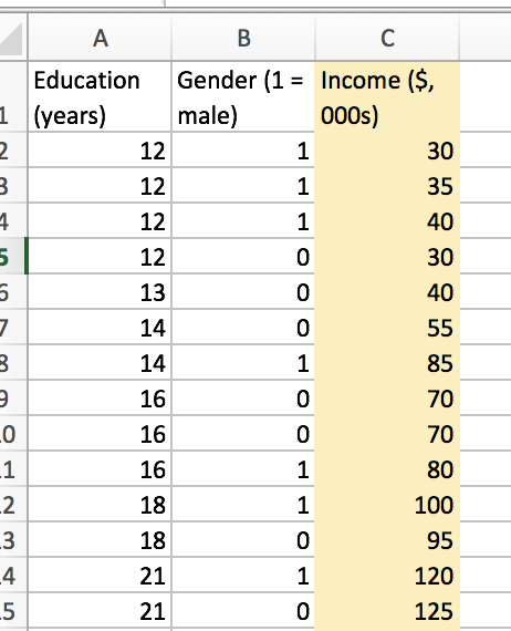
So, let’s be clear on both what this means, and how it is implemented. As always, an example would probably help. Let’s try to predict earnings from education and gender. Our data looks like this:
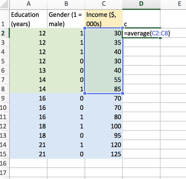
In this case, we generate a cost function, with split variable (j) and split point (s) as parameters to be optimized. Let’s split our numerical feature (years of education) at the median. Then, we’ll find the average earnings for each half plane. In this case, we split at a median of 15 (I just chose the median for funsies). I’ll use excel to find the average for region 1 and 2.
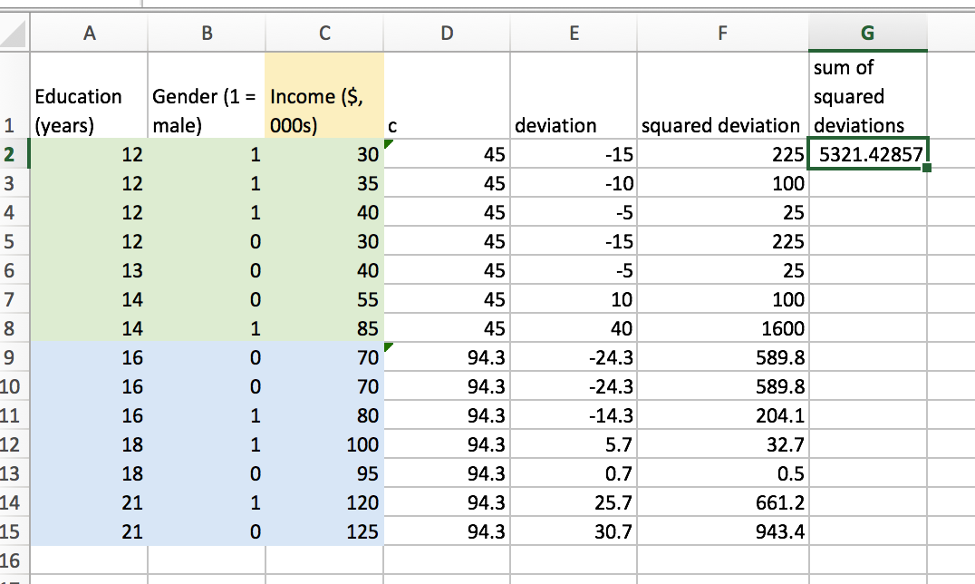
Now, we can use excel to find the sum of squared residuals for this proposed split. It looks like the following.
I am puzzled, because this doesn’t seem too computationally cheap to me. For any given split point, we need to a) find two averages, b) find the deviation for each training observation, c) square these deviations, and d) sum the squares. But, as far as I can tell, this is how things are actually done.
Part of the success of XGBoost, though, was that they altered this approach. The authors of the XGBoost package refer to this as their “Approximate Algorithm” on page 3. Ideally, I’ll get around to investigating that innovation in another post. For now, let’s move ahead to think about how we deal with categorical dependent variables.
Section 2: Categorical dependent variables
There are a lot of different methods for splitting that I read about. Vidhya analytics briefly discusses them here. In particular, 1.) Gini index, 2.) Chi square, and 3.) Information gain are addressed. I’ll talk about each here.
Gini Impurity
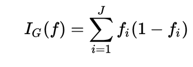
There are a few definitions of the Gini impurity thrown about, but they all get at the same idea. We’ll start with the Wikipedia definition:
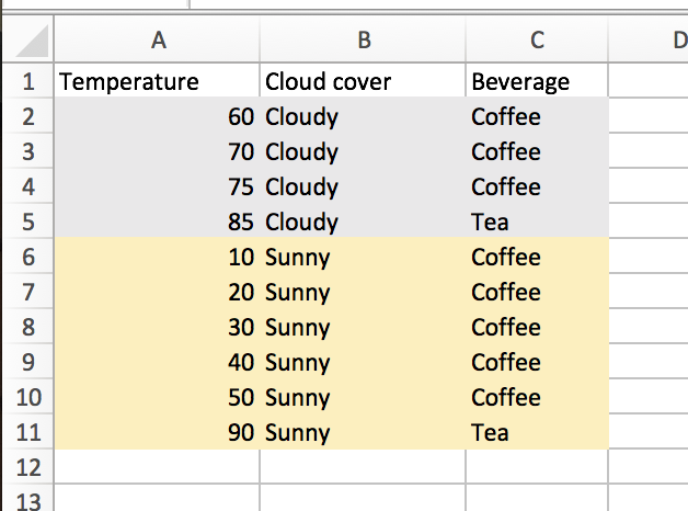
Let’s go back to the example from Part 1. We are trying to classify beverage consumption, using temperature and weather as features. Let’s focus on the weather feature to start, as it makes things simpler.
The weather decision node leads to the following splits:
Cloudy:
-
Coffee: 3/4
-
Tea: 1/4
Sunny:
-
Coffee: 5/6
-
Tea: 1/6
We find a product for each set (3/4 * 1/4 = 3/16; 5/6 * 1/6 = 5/36). Then, to find the Gini impurity for the “Cloud cover” split, we weight each product by the number of elements in each set.
In this instance, splitting on this variable and split point leads to a Gini impurity of:
(4/10)(3/16) + (6/10)(5/36) ~= .16.
This measure is fairly similar from the intuition I derived in Part 1. We look at the product of fi and (1-fi), whereas I simply considered the maximum of the two probabilities. Similarly, we weight each term in the Gini impurity by the proportion of total training observations classified in this edge of the branch. This is a similar tactic to my creation of e = log(c1)+log(c2). Both attempt to favor classication methods that broadly split the data.
Using this definition of the Gini impurity, we can consider the best and worst case scenarios. Using the above example, a split attribute that resulted in an uneven split, with classification near uniform, would be pretty bad. Let’s see how bad we can do.
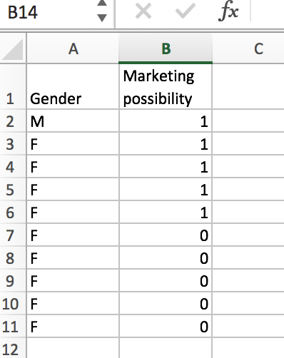
Imagine that we are trying to perform a binary classification. We are using gender as the only feature. In the following case, this would be a pretty bad scenario.
Here, we find a Gini of:
(1/10)(0/1)+(9/10)(20/81) ~= .22.
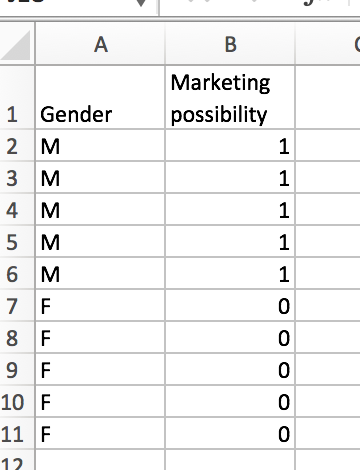
This contrasts with a similar scenario, with data more favorable to classification.
This is an ideal scenario. Splitting on gender leads to an even split of the data, and we get no impurity in our predictions from the split. The resulting Gini impurt is:
(5/10)(0/25)+(5/10)(0/25) = 0.
Other authors speak of a Gini Index, which uses a similar, but different definition. In the Gini Index, we calculate the initial scores as 1 - (fi)2 - (1-fi)2. So, using our first example, we’d find:
(4/10)(1 - (3/4)2 - (1/4)2) + (6/10)(1 - (5/6)2 - (1/6)2).
For a binary dependent variable, this measure of split quality is optimized at 1. We can see this in our Example 3. Here, we’d find (5/10)(1)+(5/10)(1) = 1.
To determine the optimal variable and split attribute, we’ll simply roll through all possibilities (all outcomes of numeric and categorical features), and choose whichever has the lowest Gini impurity.
At this point, this post has been long enough. Let’s talk through the other split metrics in future posts. In particular, I’ll address chi Square and information gain. Until next time!
As an aside, some helpful resources I used while writing this page:

