This is a continuation of the second part of a series where I intend to explain how decision trees work. In this, I will cover part 2 (How do vanilla tree algorithms really work?). Parts 3-5 will be in subsequent posts.

• Part 1: A beginner’s take on decision trees and splitting strategies.
• Part 2: How do vanilla tree algorithms actually work?
• Part 3: Why random forests are useful and what ensembles are
• Part 4: How gradient boosting applies
• Part 5: What bagging is

Section 2: Categorical dependent variables

Information gain

A populat algorithm, also known as “ID3” and developped by J. R. Quinlan, this method uses entropy calculations. At each node, we look at the entropy of the given node, and then look at the weighted, combined entropy of the new branched nodes after the split, and compare. In this algorithm, all split attributes are considered, and the greedy algorithm chooses the split with the greatest information gain. Wikipedia describes this as follows:

Let’s consider an example to make this make sense.

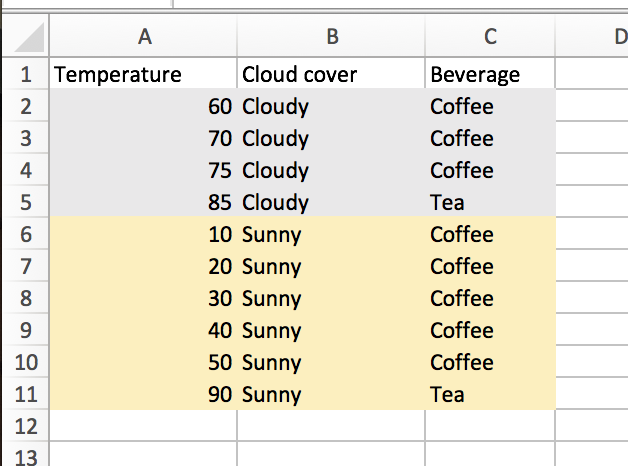
In this case, we were trying to classify beverage consumption based upon the weather. Before we split on the weather, we plainly see that 8 days had coffee consumed, and 2 days had tea. The corresponding entropy for this state (which we’ll call T₁ to match Wikipedia’s notation) is given as:

H(T₁) = -(8/10)(log(8/10)) - (2/10)(log(2/10)) ~= .72 (where logs are base 2)

When we take cloud cover into account, we should end up with a LOWER entropy. Let’s see if we do. In performing this calculation, we find the entropy of each new child node and weight according to the number of observations falling therein. We’ll call this new state T₂ and we will say that a = gender. That is, we are now classifying beverage, given that we are in a second state wherein we have conditioned on gender.

Cloudy: 4/10 days

Entropy = -(3/4)(log(3/4)) - (1/4)(log(1/4)) ~= .81

Sunny: 6/10 days

Entropy = -(5/6)(log(5/6)) - (1/6)(log(1/6)) ~= .65

Total entropy = (4/10)(.81) + (6/10)(.65) ~= .714

So we find IG = .72 - .714 = .006. Lame! This doesn’t seem like a huge information gain, and that kinda accords with out intuition. We had that most days are coffee, and tea consumption is rare. Splitting on weather isn’t really that informative, as we find that, given the weather (whether is is cloudy or sunny), the pattern of coffee dominance still holds.

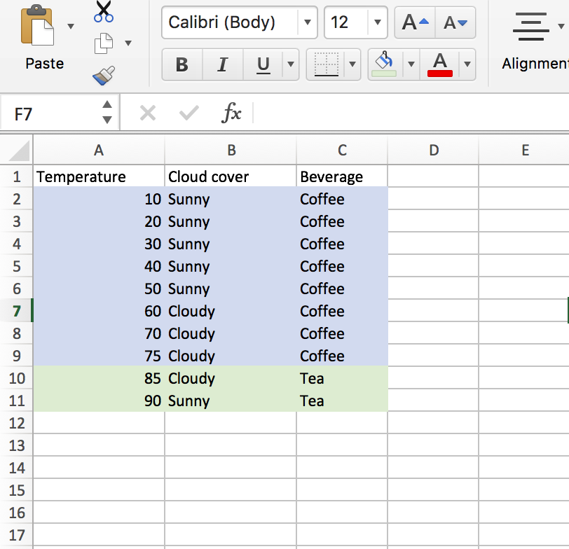
If we instead consider splitting on the numeric variable “Temperature” at a value of 80, things go much better.

After this split, we find a new entropy of…0*. So we had an information gain of .72-0 = .72. This is a much better split, and our algorithm would clearly have preferred it (judging by the IG metric). Nice!

* To see why this entropy is 0, we can see that this split attribute leads to purity in both child nodes. That is great! When performing the entropy calculations, which take the form of p(log(p)) + q(log(q)), we can tell that both products in the sum go to 0 (recall, log(1)=0).

Nice! We are cruising. Let’s look into a couple more split algorithms, and then start to move on. See you in a future post.

Citations:

Amro Wikipedia