Boosting with tree and forest classifiers
wnowak10
XGBoost is a popular ML library. It’s got the term boost in its name, so clearly the act of “boosting” is central to the performance of this algorithm. What does boosting mean with respect to decision trees and forests? Let’s investigate this issue here.
Hastie et al describe boosting as “…a procedure that combines the outputs of many “weak” classifiers to produce a powerful “committee.” As they make clear in their seminal text, the boosting algorithm (due to Freund and Schapire (1997)) successively constructs weak classifiers (meaning they are pretty randomly generated and therefore don’t do a good job of classification) on training data that differs in each successive step. In the end, we classify by weighting all of the weak classifiers according. Here’s a schematic from the ESL text.
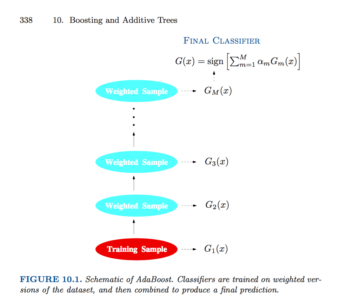
The training data changes in each step through the boosting process. We initially train on the original data, but, after each iteration, we adjust the training data, and give more weight to the observations that were previously misclassified. In this way, we boost hard to classify observations.
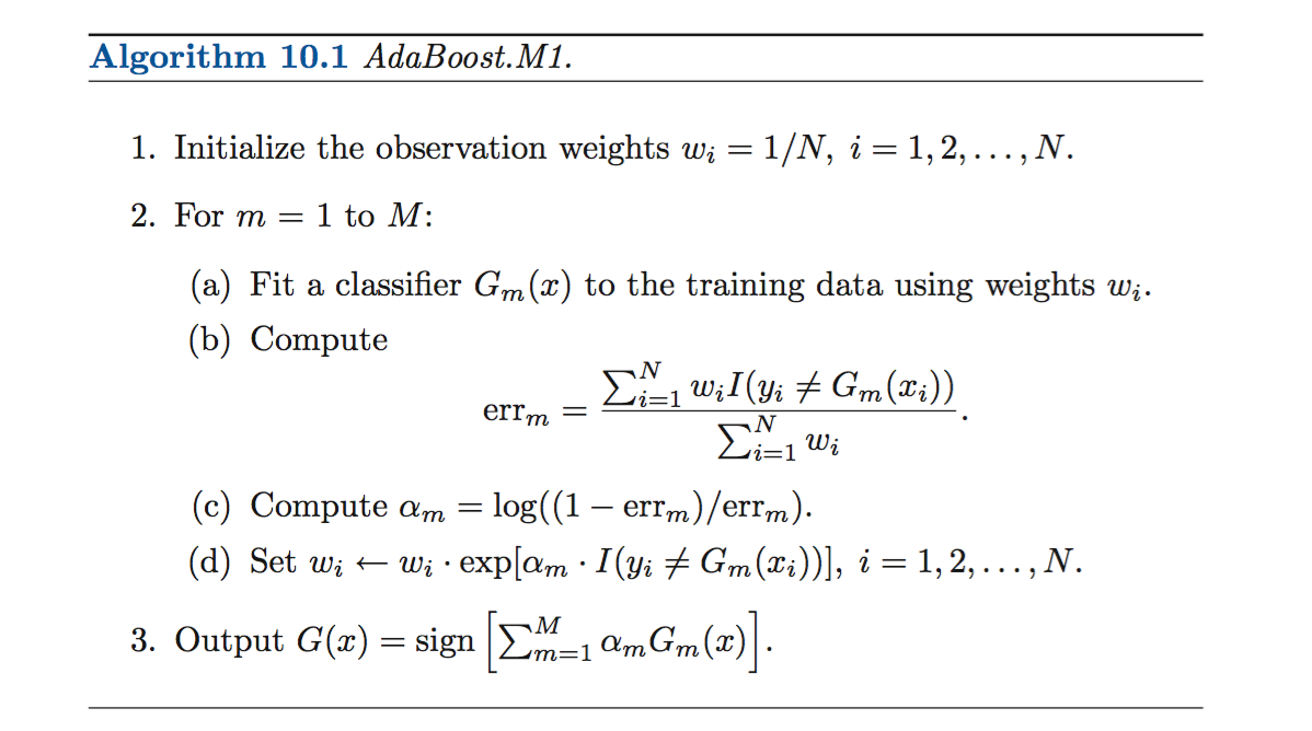
ESL outlines the pseudo-algorithm here:
As in the post on forests, I will try to recreate the simulation Hastie et al run.
Generate data
First, we generate the training and test data.
#make_boost_data

#boosting from ESL p. 339
# create train data creation function. n = # obs= user input

create_train_data = function(n){
  # create features x1 through x10 (random normal)
  for(i in 1:10){
  	# use assign function to create variable names (x1, x2...)
    assign(paste("x", i, sep = ""), rnorm(n))
  }

  # create label vay (y) as per ESL p. 339 (eq. 10.2)
  y_lim=qchisq(.5,10)
  y=ifelse(x1^2+x2^2+x3^2
           +x4^2+x5^2+x6^2
           +x7^2+x8^2
           +x9^2+x10^2>y_lim,1,-1)

  # combine into df
  df = data.frame(x1,x2,x3,x4,
                  x5,x6,x7,x8,
                  x9,x10,y)
  # make y as factor for rpart class prediction
  df$y=as.factor(df$y)
  return(df)
}

# create test data creation function. same as train data generation
create_test_data = function(n_test){
  # create features
  for(i in 1:10){
    assign(paste("x", i, sep = ""), rnorm(n_test))
  }

  # create label var (y)
  y_lim=qchisq(.5,10)
  y=ifelse(x1^2+x2^2+x3^2
           +x4^2+x5^2+x6^2
           +x7^2+x8^2
           +x9^2+x10^2>y_lim,1,-1)

  df = data.frame(x1,x2,x3,x4,
                  x5,x6,x7,x8,
                  x9,x10,y)
  df$y=as.factor(df$y)
  return(df)
  # sum(y==1) # should be around 1000 according to ESL.
  # it is
}
Fit initial model
If we use a 1 stump classifier, we can see the results on the test set match the ESL text. We use the R rpart library’s rpart function to fit a tree. We fit y on all features (x1…xn), using the “class” method (is classification and not regression). We use our train_df created by the create_train_data function as our training observations. We use the rpart.control option to limit the depth of the tree to 1. We are creating stumps.

library(rpart)
fit <- rpart::rpart(y ~ x1+x2+x3+x4+x5+
               x6+x7+x8+x9+x10,
             method="class", data=train_df,
             control=rpart.control(maxdepth=1))
If we use rpart.plot, we can see what this stump looks like.
library(rpart.plot)
rpart.plot(fit,type=0)
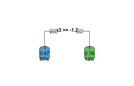
To understand what this image shows…
- If x3>= 1.2, we predict y=-1. .47=47% of our training data was classified this way, and the accuracy when following that rule is 87% (e.g. 87% of y values in our training set =-1, when x3>=-1.2).
- Else, we predict y=1 (with a similar explanation applying).
(FYI - this is a pretty bad fitting model. We can see from the data generating function that one single split won’t do well to model the data, so here a fairly arbitrary split is made.)
Error rates
We then create functions to return the error rates when fed a model and data. We split the train error function into two, as it will be useful to have a unique function to spit out predictions when we try to implement algorithm 10.1.
# function to generate predicted y values, given a model (fit) and test data
predictions = function(fit,train_df){
  # predict function with "vector" type returns 1,2 as outputs (corresponding to #-1 and 1)
  train_p=predict(fit,newdata=train_df,type="vector")
  # replace to match -1 and 1 with training label
  train_p=replace(train_p, train_p==1, -1)
  train_p=replace(train_p, train_p==2, 1)
  return(train_p)
}

# given predictions and class labels...report error rate
train_error_rate = function(train_p,train_df){
  train_success=sum(train_p==train_df$y)/length(train_p)
  return(1-train_success) # train success rate
}

# redundant function...do above functions, in 1
test_error_rate = function(fit,test_df){
  p=predict(fit,newdata=test_df,type="vector")
  # codes 0s as 2s for some reason
  # run this in order!
  p=replace(p, p==1, -1)
  p=replace(p, p==2, 1)
  #head(p)
  #head(test_df$y)
  test_success = sum(p==test_df$y)/length(p) # test success!
  return(1-test_success) # test error rate matches ESL
}

predictions(fit,train_df)
train_error_rate(fit,train_df)
test_error_rate(fit,tes_df)
Now, we implement the algorithm.

# create empty lists for errm, alpham, and predictions at each step through
err=c()
alpha=c()
preds=c()

# function to return boosted model
# take m = number of boosting iterations, training data and testing data
# as inputs

boost = function(m,train_df,test_df){
  # how big is training data?
  n = nrow(train_df)
  # create weights
  w = rep(1/n,n) #where n is number of training obs

  # repeat boosting alg (10.1) m times
  for(i in seq(m)){
    # set training_df to take into account weights
    boost_fit <-rpart(y ~ x1+x2+x3+x4+x5+
                          x6+x7+x8+x9+x10,
                          method="class", data=train_df,
                          weights = w,
                          control=rpart.control(maxdepth=1))
    # load predictions function.
    source('predict_error.R')
    # generate predicted values on test set, given most recent fit (G)
    # store in list pred
    preds=c(preds,predictions(boost_fit,test_df))

    predictions=predictions(boost_fit,train_df) # find predictions on train to keep working on model

    # use matrix multiply to find sigma of products
    err=c(err,(w%*%(predictions!=train_df$y)) / (sum(w)) )
    # in line above, we are finding sigma (wi * indicator function)
    # what we are doing is finding the weighted error.
    # finding predictions!=train_df$y gives errors, so the initial
    # round is just the raw error rate. subsequent rounds are weighted error rates

    alpha=c(alpha,log((1-err[i])/(err[i]))) # reference first error (i=1)
    # if error rate high, this approaches neg inf
    # if error rate low (near 0), this approaches + inf

    numeric_mismatch=as.numeric(predictions!=train_df$y)
    w = w*exp(alpha[i]*numeric_mismatch) # set new weights
    # if we missed prediction, w changes to w* e^alpha. if error rate
    # was high, this was like e^-inf = 0...that doesnt make sense?

  }
  # how many rows are in test set?
  num_test_obs=dim(test_df)[1]

  summ=rep(0,num_test_obs)
  chunks = list()
  for(i in 1:m){
  	# generate list of siz num_test_obs that contains predictions
    chunks[[i]] = preds[(1+((i-1)*num_test_obs)) : (num_test_obs+((i-1)*num_test_obs))]
    # add running weighted  sum of predictions. this is step 3 in alg. 10.1
    summ = summ+alpha[i]*chunks[[i]]
  }
  # finish and return predicted values
  vals=ifelse(summ>0,1,-1)
  return(vals)
}
Let’s work through this step by step. First we create empty lists for us to compute errm and alpham. In the boost function, we initialize the weights, so every observation has weight 1/n (with n the number of obs). Then, we enter the for loop as per line 2.
For 2a), we fit a stump:
boost_fit <- rpart(y ~ x1+x2+x3+x4+x5+
                   x6+x7+x8+x9+x10,
                 method="class", data=train_df,
                 weights = w,
                 control=rpart.control(maxdepth=1)) # fit initial tree
For 2b), we compute errm. To find the sum of wi * I, we use matrix multiplication to find the dot product. To generate the indicator function (such that I = 1 when we have MISpredicted, we run the following):
predictions!=train_df$y
For 2c), we compute alphai. If we correctly predict, w stays the same )w = wexp(0)). If we mispredict, then we multiple wlog((1-err)/err). This has the effect of making w larger when our error approaches 0.
alpha=c(alpha,log((1-err[i])/(err[i]))) # reference first error (i=1)
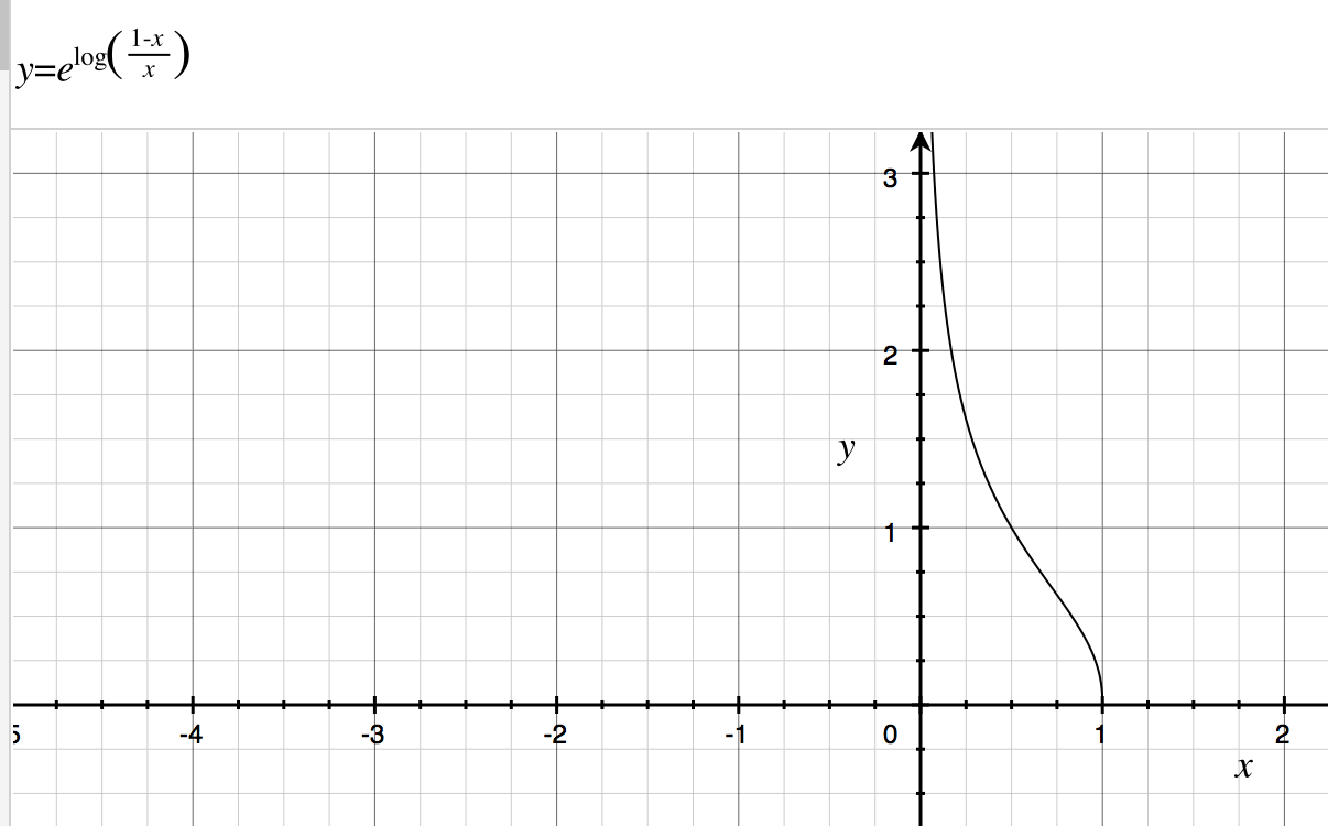
w = w*exp(alpha[i]*numeric_mismatch) # set new weights
The last bit of code adds the predictions at each step. We take preds, which is a long list of predictions (nrow(test_df)*m) and split this back up into m lists of size nrow(test_df). Then we weight by alpha and sum. We return the predicted values for test_df, found when trained with train_df.
HSL find the following with this data and their simulations.
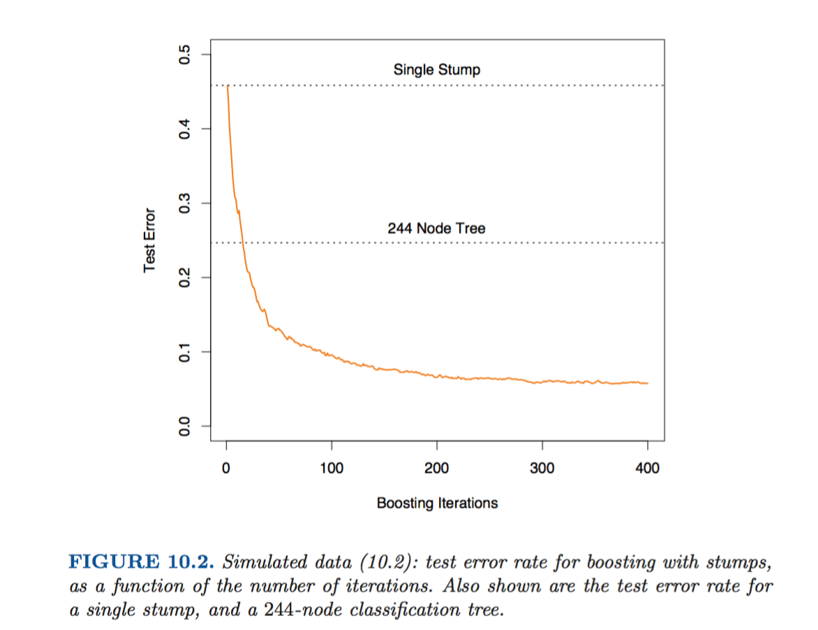
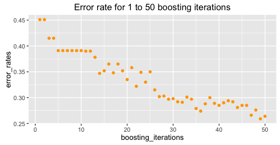
When I recreate (and lower boosting iterations, as running for 1:400 iterations takes a bit long), I find:
